BASIC

The winLIFE BASIC module covers the essential basics of analytical fatigue life prediction. Typically, winLIFE users start their work with this module. The following extensions are available for the BASIC module, which can be purchased additionally:

winLIFE MULTIAXIAL

winLIFE MULTIAXIAL MULTICORE

winLIFE GEARWHEEL&BEARING

winLIFE CRACKGROWTH

winLIFE VIEWER4WINLIFE

winLIFE RANDOM FATIGUE

winLIFE STATISTIC

winLIFE Project Management System

Typical industrial tasks involve not only a single analytical fatigue life prediction, but usually a large number of load cases and variants.

For this purpose, winLIFE offers a powerful project management system that can handle up to 2000 projects simultaneously. The picture below shows the user interface where 8 projects are defined. The projects can be edited individually, but they can also be started together and superimposed.

A project generator enables the generation of projects in which individual parameters can be systematically varied.

As many calculations lead to long computing times, an automated process is important, so that the possibility of batch processing is of great importance. The project files are saved in XML format and can also be started as a batch from the user interface.

How do I obtain Material Data for an Analytical Fatigue Life Prediction?

winLIFE offers several options for obtaining material data for the analytical fatigue life prediction. In addition to generation based on static material data, extensive material databases are included in the scope of delivery.

Generation of S-N Curves from Static Material Data

As winLIFE has many customers in the wind energy, shipbuilding and general engineering sectors, special input generators have been created to generate fatigue life data from static material parameters. These are

• S-N curve generator for welded joints according to Germanischer Lloyd for shipbuilding
• S-N curve generator for welded joints according to Germanischer Lloyd for wind turbines
• S-N curve generator for welded joints according to the FKM-guideline
• S-N curve generator according to Hück, Trainer, Schütz
• Generator according to Uniform Material Law

The following figure shows an example of an input mask for a generator according to the FKM guideline, which is based on a wealth of experience and is already established in many areas. The S-N curve can be estimated from static material data such as yield strength, tensile strength and component information such as surface, notch factor, stress gradient, etc.

The figure above shows the input screen used to generate these S/N-curves. Once generated, the user can partially overwrite the data to modify known individual values.

In addition to the S-N curve, the Haigh diagram is also used to provide more comprehensive information, as it also shows the mean stress sensitivity and the yield and break points (see next figure).

If the probability of failure is important to an investigation, any number of S-N curves with different probabilities of failure can be derived from the 50% S-N curve, taking into account different scatters in the range of fatigue strength for finite life and fatigue limit.

S-N Curves defined Point by Point (ASME CODE)

The S-N curve of a component is defined by a large number of individual points between which interpolation takes place. This definition of the S-N curve has now been implemented in winLIFE at the the customer's request. The following example shows such a S-N curve.

Generation of component S-N curves for welded components

Component S-N curves can be generated in accordance with the FKM, Germanischer Lloyd (shipbuilding, wind energy), IIW guidelines. Fatigue life can be calculated according to the nominal stress concept or the structural stress concept.

The geometry and notch factors are taken into account by assigning them to a catalogue of different weld seams (detail classes, FAT classes).

Powerful macros for FEMAP and ANSYS are available for data transfer to winLIFE.

GENERATION OF STRAIN S-N CURVES

Strain S-N curves can be generated from static material characteristics. In addition to the most commonly used Uniform Material Law, other algorithms are available.  The procedure is shown in the figure below: Static material characteristics are specified (right-hand side) and the material characteristics for the S-N curve and the cyclic behaviour are generated from them (left-hand side).

The following figure shows a calculation example where the cyclic data was obtained and displayed by generating it from the static characteristic values. The shape factor and surface roughness in the notch have been specified for the component. The stress-strain curve in the notch is calculated for the component from the rainflow matrix. The curve can also be calculated directly from the material memory without rainflow counting.

Material Databases

The following material databases are supplied with the installation:

Material database for the local concept
Material database according to FKM
User database

Material Database for the Local Strain Concept

An extensive database (more than 1000 materials) with the following
information is available for calculations according to the local concept:

• Static material characteristics
• Cyclic material characteristics
• General information and, in particular, information sources

Own data can be integrated into the database.

Material Database for Calculation according to FKM

Common material data from trial tests can be taken from the supplied database with data from the FKM guideline.
This data can be used to generate S-N curves for the component.

By entering the component data in addition to the material data, a component S-N curve can be generated and stored in the user database.

User Database

The winLIFE user saves the material/component data used for the fatigue life calculation in a user database containing the material and component information.

Obtaining the Load Data

For a fatigue life calculation, data on the acting load is required. This can be a measured load-time curve or a frequency distribution of loads (load spectrum).

Definition of a Load Spectrum

A load spectrum is defined by the following triplet of values

• Mean load
• Load amplitude
• Number of cycles

Experience in various fields of engineering shows that the acting load spectra have certain basic forms that are easy to describe. If you know the basic form of the acting load spectra - e.g. from publications - you can easily generate a load spectrum adapted to the individual component with the winLIFE spectrum generator.  The following figure shows three such basic forms of load spectra generated with winLIFE.

USING LOAD-TIME HISTORIES

Another way of describing loads is to use load-time histories. A load can be a stress, a torque or a force. Such data can be obtained from measurements, but it is also possible for the user to enter the load-time curve manually using the keyboard. Alternatively, the sine generator can be used to easily generate load-time functions.

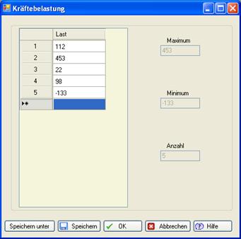
Loads (Manual Input)

Loads - e.g. forces as a function of time - are entered in the input screen and then saved. For time reasons, only short load sequences are entered in this way.

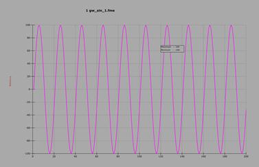
Force Generator (Sine Curve)

It is often required to generate simple load-time curves quickly and easily. This is possible with the sine curve generator described here.

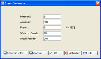
The entries should be self-explanatory. The result of the generation looks like this:

Import of Measured Load-Time Functions

In most cases, very large measurement data is used, which can be several gigabytes in size.

Interactive data post-processing in the graph allows easy correction of the load-time history or load spectrum data. For example, spikes can be quickly removed and corrections made to signal drift.

The rainflow matrix used by winLIFE can also be post-processed. The rainflow matrix contains the damage-relevant events and displays their degree of damage using a colour scale. By changing the rainflow matrix, alternative load scenarios can be easily simulated.

In the local concept, the stress-strain curve can be visualised. It is visualised from the rainflow matrix and the cyclic material characteristics.

ANALYSIS IN THE FREQUENCY RANGE

The natural frequencies of a dynamically excited system and the frequency spectrum of the excitation have a major influence on the fatigue life. It is therefore very useful to determine the stresses acting on a component using the Power Density Spectrum (PSD). Components are often tested on an oscillating table using this PSD of acceleration. winLIFE RANDOM does exactly this. The module is introduced in a separate chapter.

Using FEA

When using an FE model, a unit load case is calculated using the FEM. winLIFE BASIC is limited to one unit load case. (winLIFE MULTIAXIAL can calculate up to 200 load cases simultaneously). For details on data transfer, see winLIFE MULTIAXIAL.

Procedure based on an example

The procedure of a fatigue life calculation with winLIFE BASIC is now briefly described. This is done using the example of a control arm of a truck wheel suspension, which is loaded with a measured load-time function. For reasons of symmetry, only the upper half of the component is shown.

In the first step, a static FEA using the unit load F_o  is required. It is important that the unit load has the same line of action as the operational load F(t).

For each time step t, the elastic stress (more correctly the stress tensor) is calculated as a result of the load F(t) using the quotient F(t)/F_o. If a time history F(t) as shown in the following figure is available, the stress in the component can be calculated for each desired time step.

When using the local concept, a stress-strain curve is available which is included in the calculation. In this way, the plasticisation of the material is also taken into account with the help of the Neuber rule.

 
The component load (figure above) was obtained from a measurement on a test track. winLIFE now performs a rainflow count of the load, the result of which is shown in the following figure.

The cyclic material data and the S-N curve of the damage parameters for this example are shown in the two figures below.

The stress-strain path is constructed from the rainflow matrix and the cyclic material data. The closed loops of this path are used to calculate a damage parameter and the damage is finally determined for each node of the structure using the damage parameter S-N curve. The results are visualised as areas of equal damage on the structure.

In addition to the local concept, a stress-based concept can also be used for the calculation, using stress-based S-N curves.

The results of the fatigue life calculation: damage sum, damage equivalent amplitude and number of load cycles to failure are output to an export file. The FE programme accesses this export file and is displayed as shown in the following figure. An interface is provided for FEMAP, which is automatically installed in the FEMAP user interface.

Without FEA

If finite elements are not used, the fatigue life calculation is performed for only one point, usually the notch. Information about the geometry and the load/stress relationship must then be provided by the user, i.e. notch factor, stress gradient, surface roughness, etc. must be specified. A fatigue life calculation without finite elements can be performed according to the two classical methods, the nominal stress concept or the local concept.

In the nominal stress approach, different hypotheses for damage accumulation in the area of the fatigue limit can be used (original, modified Haibach, elementary, modified Liu and Zenner). The following figure shows the available hypotheses.

If the calculation is performed according to the local concept, the procedure is similar to the application of the finite element method, except that only one point is calculated.

Addition of different Calculation Results

Suppose you are developing a car that will naturally be used on very different road categories (good road, bad road, etc.).

If fatigue life measurements and calculations are available for each road category, but their length does not match the client's route, the fatigue life results must be converted to the client's route composition. This is done by converting the results (damage sum per road category) to the desired route length using weighting factors and adding them up for each node and section level.

Since for many tasks very different scenarios have to be analysed and then discussed in terms of their overall impact, weighted addition is an important tool, as smaller sub-problems can be dealt with first.

Superposition and Extrapolation

In contrast to the simple addition of calculation results - as described in the previous chapter - it is often important to know the total spectrum in order to better interpret the results.
The addition of several consecutive partial loads (spectra) is called superposition.
The conversion of the measured partial load of e.g. 500 h to the total load of 20 years is called extrapolation.

Table: Data of a test drive with target and actual values and the factor calculated for the extrapolation.

Statistical Analysis

The following input screen is provided for the statistical analysis of the reliability probability. The results of the previous fatigue life calculation and the data of the used S-N curve are taken over.

The S-N curve data

• Scatter range
• Number of test points n

are accepted. They can be subsequently modified by the user in this screen.
The user now has to enter the confidence level and the probability of occurrence of his collective. When the user clicks on Calculate, the following result is obtained

• the true arithmetic probability of default PA
• the simplified probability of default PA*.

Data Processing and Correction

When using measurement data, it is usually necessary to clean the data. Many possible errors can occur and in the first step of an analysis the user must check and usually also correct his measurement data. winLIFE allows simple and fast interactive correction of the data.

Load-time functions and load spectra can be corrected as follows

• Selecting data and correcting the selected data by multiplying, adding or overwriting
• Finding and removing spikes

The Rainflow matrix can also be modified. This is also very useful when performing data correction.

Display and Analysis of Results

All common graphics and visualisations are available in winLIFE, such as

• Rainflow-Matrix
• Range pair mean counting
• Level crossing counting
• S-N-Curve with load spectrum and associated damage proportion
• Haigh diagram including the value triples of the stresses
• Log file with the results for each individual node

Report Generator

The Report Generator allows the user to generate a standard report in PDF format, including graphics, at the touch of a button. This eliminates the need to select each graphic individually.

The standard report is defined differently for each method, but can be modified by the user.

CUSTOMISED DESIGN OF GRAPHICS AND REPORTS

The design of the output documents, in particular the graphics, can be customised by the user with regard to the following parameters

• Font size and font type
• Line colour
• Line style and line thickness
• Range setting of the axes
• Text input

The unit of the stresses can be defined by the user in various ways. The internal calculation in winLIFE is carried out in N/mm². If a different unit is required, this can be selected from the unit list. PSI is usually requested as an alternative, so that this unit is prepared.
However, any unit can also be defined by the user by specifying the name and the multiplier for the conversion.
The other units used in winLIFE are the following and cannot be changed.

• Strain [‰]
• RPM [1/min]